Pregunta: (17-4 y 17-5) a) Explore la respuesta de la tasa de adquisición a diferentes magnitudes para el incremento escalonado del stock de capital deseado. ¿Cómo afecta el tamaño del incremento a la tasa de ajuste del stock de capital al nuevo equilibrio? ¿Depende la razón de amplificación de la tasa de adquisición del tamaño del incremento del capital deseado? ¿Por

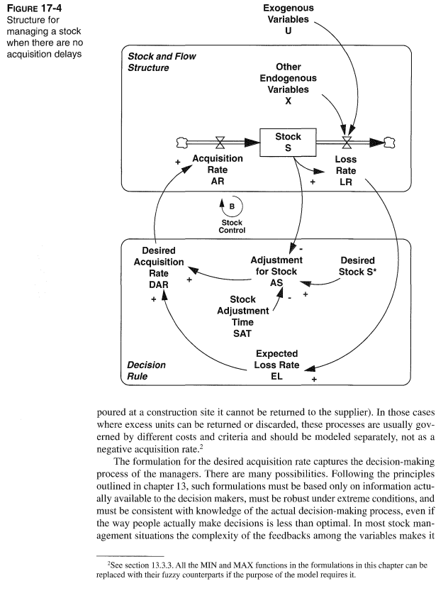
17.2.1 Managing a Stock: Structure The stock management control problem can be divided into two parts: (1) the stock and flow structure of the system and (2) the decision rule used by the managers to control the acquisition of new units. To begin, consider a situation in which the manager controls the inflow rate to the stock directly and there is no delay in acquiring units (Figure 17-4). ${}^1$ Filling a glass of water from a faucet provides an example: The delay between a change in the state of the system (the level of water in the glass) and the inflow to the stock (the rate at which water flows from the tap) is short enough relative to the flow that it can safely be ignored. The stock to be controlled, S , is the accumulation of the acquisition rate AR less the loss rate LR: $\mathrm{S}=\mathrm{INTEGRAL}\left(\mathrm{AR}-\mathrm{LR},{\mathrm{S}}_6\right)$ Losses include any outflow from the stock and may arise from usage (as in a raw material inventory) or decay (as in the depreciation of plant and equipment). The loss rate must depend on the stock itself-losses must approach zero as the stock is depleted-and may also depend on sets of other endogenous variables $\mathbf{X}$ and exogenous variables $\mathbf{U}$. Losses may be nonlinear and may depend on the age distribution of the stock: $\mathrm{LR}=f(\mathbf{S},\mathbf{X},\mathbf{U})$ How should the acquisition rate be modeled? In general, managers cannot add new units to a stock simply because they desire to do so. First, the acquisition of new units may involve time delays. Second, the acquisition of new units for a stock usually requires resources: Production requires labor and equipment; hiring requires recruiting effort. These resources may themselves be dynamic. The resources available at any moment impose capacity constraints. For now, assume the capacity of the process is ample and that there are no significant time delays in acquiring new units. Therefore the actual acquisition rate, $AR$, is determined by the desired acquisition rate, DAR: $\mathrm{AR}=\mathrm{MAX}(0,\mathrm{DAR})$ The MAX function ensures that the acquisition rate remains nonnegative. In most situations, the acquisition rate cannot be negative (once concrete is delivered and ${}^1$ The discussion assumes the manager controls the inflow to the stock and must compensate for changes in the outflow. There are many stock management situations in which the manager's task is to adjust the outflow from a stock to compensate for changes in the inflow. A firm must adjust shipments to keep its backlog under control as orders vary; managers of a hydroelectric plant must adjust the flow through the dam to manage the level of impounded water as the inflow varies. The principles for stock management in these situations are analogous to those for the case where the managers control the inflow alone. Figure 17-4 Structure for managing a stock when there are no acquisition delays poured at a construction site it cannot be returned to the supplier). In those cases where excess units can be returned or discarded, these processes are usually governed by different costs and criteria and should be modeled separately, not as a negative acquisition rate. ${}^2$ The formulation for the desired acquisition rate captures the decision-making process of the managers. There are many possibilities. Following the principles outlined in chapter 13, such formulations must be based only on information actually available to the decision makers, must be robust under extreme conditions, and must be consistent with knowledge of the actual decision-making process, even if the way people actually make decisions is less than optimal. In most stock management situations the complexity of the feedbacks among the variables makes it ${}^2$ See section 13.3.3. All the MIN and MAX functions in the formulations in this chapter can be replaced with their fuzzy counterparts if the purpose of the model requires it. loop. The simplest formulation is to assume the adjustment is linear in the discrepancy between the desired stock ${\mathrm{S}}^{\ast }$ and the actual stock: $\mathrm{AS}=\left({\mathrm{S}}^{\ast }-\mathrm{S}\right)/\mathrm{SAT}$ where ${\mathrm{S}}^{\ast }$ is the desired stock and SAT is the stock adjustment time (measured in time units). The stock adjustment forms a linear negative feedback process. The desired stock may be a constant or a variable. 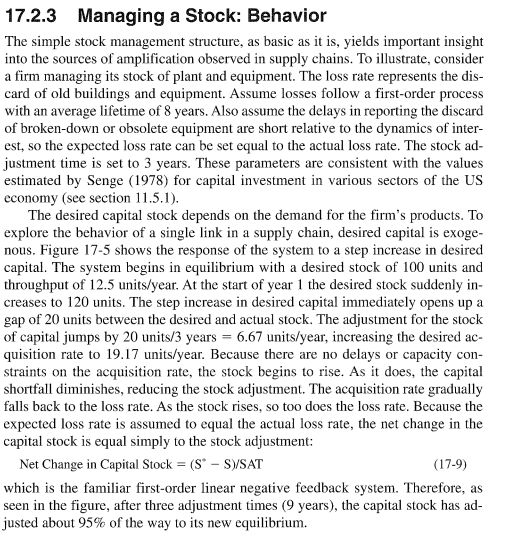17.2.3 Managing a Stock: Behavior The simple stock management structure, as basic as it is, yields important insight into the sources of amplification observed in supply chains. To illustrate, consider a firm managing its stock of plant and equipment. The loss rate represents the discard of old buildings and equipment. Assume losses follow a first-order process with an average lifetime of 8 years. Also assume the delays in reporting the discard of broken-down or obsolete equipment are short relative to the dynamics of interest, so the expected loss rate can be set equal to the actual loss rate. The stock adjustment time is set to 3 years. These parameters are consistent with the values estimated by Senge (1978) for capital investment in various sectors of the US economy (see section 11.5 .1 ). The desired capital stock depends on the demand for the firm's products. To explore the behavior of a single link in a supply chain, desired capital is exogenous. Figure $17-5$ shows the response of the system to a step increase in desired capital. The system begins in equilibrium with a desired stock of 100 units and throughput of 12.5 units/year. At the start of year 1 the desired stock suddenly increases to 120 units. The step increase in desired capital immediately opens up a gap of 20 units between the desired and actual stock. The adjustment for the stock of capital jumps by 20 units $/3$ years $=6.67$ units/year, increasing the desired acquisition rate to 19.17 units/year. Because there are no delays or capacity constraints on the acquisition rate, the stock begins to rise. As it does, the capital shortfall diminishes, reducing the stock adjustment. The acquisition rate gradually falls back to the loss rate. As the stock rises, so too does the loss rate. Because the expected loss rate is assumed to equal the actual loss rate, the net change in the capital stock is equal simply to the stock adjustment: Net Change in Capital Stock $=\left({\mathrm{S}}^{\ast }-\mathrm{S}\right)/$ SAT which is the familiar first-order linear negative feedback system. Therefore, as seen in the figure, after three adjustment times ( 9 years), the capital stock has adjusted about $95\%$ of the way to its new equilibrium. Figure 17-5 Response to a step increase in the desired stock The consequences of the stock management structure for supply chain management are profound. First, the process of stock adjustment creates significant amplification. Though the desired stock increased by $20\%$, the acquisition rate increases by a maximum of more than $53\%$ (the peak acquisition rate divided by the initial acquisition rate $=19.2/12.5$ ). The amplification ratio (the ratio of the maximum change in the output to the maximum change in the input) is therefore $53\%/20\%=2.65$. A $1\%$ increase in desired capacity causes a $2.65\%$ surge in the demand for new capital. While the value of the amplification ratio depends on the stock adjustment time and capital lifetime, the existence of amplification does not. A longer adjustment time reduces the size of the adjustment for the stock for any given discrepancy between the desired and actual stocks and thus reduces amplification, but also lengthens the time required to close the gap and reach the new goal. Second, amplification is temporary. In the long run, a $1\%$ increase in desired capital leads to a $1\%$ increase in the acquisition rate. But during the disequilibrium adjustment, the acquisition rate overshoots the new equilibrium. The overshoot is an inevitable consequence of the stock and flow structure. The only way a stock can increase is for the acquisition rate to exceed the loss rate. The acquisition rate must increase above the loss rate long enough to build up the stock to the new desired level. The firm's suppliers face much larger changes in demand than the firm itself and much of the surge in demand is temporary.